SIFT算法分析报告

《SIFT算法分析报告》由会员分享，可在线阅读，更多相关《SIFT算法分析报告（13页珍藏版）》请在装配图网上搜索。

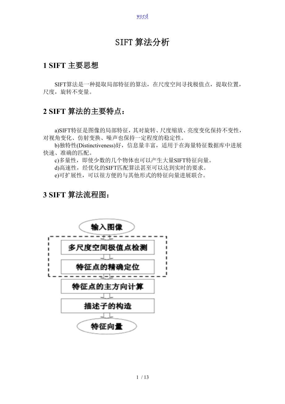
1、word SIFT算法分析 1 SIFT主要思想 SIFT算法是一种提取局部特征的算法，在尺度空间寻找极值点，提取位置，尺度，旋转不变量。 2 SIFT算法的主要特点： a)SIFT特征是图像的局部特征，其对旋转、尺度缩放、亮度变化保持不变性，对视角变化、仿射变换、噪声也保持一定程度的稳定性。 b)独特性(Distinctiveness)好，信息量丰富，适用于在海量特征数据库中进展快速、准确的匹配。 c)多量性，即使少数的几个物体也可以产生大量SIFT特征向量。 d)高速性，经优化的SIFT匹配算法甚至可以达到实时的要求。 e)可扩展性，可以很方便的与其他形式的特征向量进展联

2、合。 3 SIFT算法流程图： 4 SIFT算法详细 1〕尺度空间的生成 尺度空间理论目的是模拟图像数据的多尺度特征。 高斯卷积核是实现尺度变换的唯一线性核，于是一副二维图像的尺度空间定义为： 其中 是尺度可变高斯函数， 〔x，y〕是空间坐标，是尺度坐标。大小决定图像的平滑程度，大尺度对应图像的概貌特征，小尺度对应图像的细节特征。大的值对应粗糙尺度(低分辨率)，反之，对应精细尺度(高分辨率)。 为了有效的在尺度空间检测到稳定的关键点，提出了高斯差分尺度空间〔DOG scale-space〕。利用不同尺度的高斯差分核与图像卷积生成。 DOG算子计算简单，

3、是尺度归一化的LoG算子的近似。 图像金字塔的构建：图像金字塔共O组，每组有S层，下一组的图像由上一组图像降采样得到。 图1由两组高斯尺度空间图像示例金字塔的构建，第二组的第一副图像由第一组的第一副到最后一副图像由一个因子2降采样得到。图2 DoG算子的构建： 图1 Twooctavesof aGaussian scale-spaceimagepyramid with s =2 intervals. The first imageinthe second octaveis createdbydown samplingtolastimageintheprevious 图2 The

4、 difference of two adjacent intervals in the Gaussian scale-space pyramid create anintervalinthedifference-of-Gaussianpyramid(showningreen). 2)空间极值点检测 为了寻找尺度空间的极值点，每一个采样点要和它所有的相邻点比拟，看其是否比它的图像域和尺度域的相邻点大或者小。如图3所示，中间的检测点和它同尺度的8个相邻点和上下相邻尺度对应的9×2个点共26个点比拟，以确保在尺度空间和二维图像空间都检测到极值点。 一个点如果在DOG尺度空间本层以与上下两层的2

5、6个领域中是最大或最小值时，就认为该点是图像在该尺度下的一个特征点,如图1所示。 图3 DoG尺度空间局部极值检测 3)构建尺度空间需确定的参数 －尺度空间坐标 O－octave坐标 S－ sub-level 坐标 和O、S的关系， 其中是基准层尺度。o－octave坐标，s－ sub-level 坐标。注：octaves 的索引可能是负的。第一组索引常常设为0或者-1,当设为-1的时候，图像在计算高斯尺度空间前先扩大一倍。 空间坐标x是组octave的函数，设是0组的空间坐标，如此 如果是根底组o=0的分辨率，如此其他组的分辨率由下式获得： 注

6、：在Lowe的文章中，Lowe使用了如下的参数： 在组o=-1，图像用双线性插值扩大一倍〔对于扩大的图像〕。 4〕准确确定极值点位置 通过拟和三维二次函数以准确确定关键点的位置和尺度〔达到亚像素精度〕，同时去除低比照度的关键点和不稳定的边缘响应点(因为DoG算子会产生较强的边缘响应)，以增强匹配稳定性、提高抗噪声能力。 ①空间尺度函数 〕泰勒展开式如下: 对上式求导,并令其为0,得到准确的位置, ②在已经检测到的特征点中,要去掉低比照度的特征点和不稳定的边缘响应点。去除低比照度的点：把公式(4)代入公式(3)，只取前两项可得： 假如，该特征点就保存下来，否如此丢弃。

7、 ③边缘响应的去除 一个定义不好的高斯差分算子的极值在横跨边缘的地方有较大的主曲率，而在垂直边缘的方向有较小的主曲率。主曲率通过一个2x2 的Hessian矩阵H求出: 导数由采样点相邻差估计得到。 D的主曲率和H的特征值成正比，令为最大特征值，为最小的特征值，如此 令，如此： (r + 1)2/r的值在两个特征值相等的时候最小，随着r的增大而增大，因此，为了检测主曲率是否在某域值r下，只需检测 在Lowe的文章中，取r＝10。 5〕关键点方向分配 利用关键点邻域像素的梯度方向分布特性为每个关键点指定方向参数，使算子具备旋转不变性。 式(5)为(x,y

8、)处梯度的模值和方向公式。其中L所用的尺度为每个关键点各自所在的尺度。 在实际计算时，我们在以关键点为中心的邻域窗口采样，并用直方图统计邻域像素的梯度方向。梯度直方图的围是0～360度，其中每10度一个柱，总共36个柱。直方图的峰值如此代表了该关键点处邻域梯度的主方向，即作为该关键点的方向。图4是采用7个柱时使用梯度直方图为关键点确定主方向的示例。〔窗口尺寸采用Lowe推荐的σ×σ〕 图4由梯度方向直方图确定主梯度方向 在梯度方向直方图中，当存在另一个相当于主峰值80%能量的峰值时，如此将这个方向认为是该关键点的辅方向。一个关键点可能会被指定具有多个方向〔一个主方向，一个以上辅方向〕

9、，这可以增强匹配的鲁棒性[53]。 至此，图像的关键点已检测完毕，每个关键点有三个信息：位置、所处尺度、方向。由此可以确定一个SIFT特征区域〔在实验章节用椭圆或箭头表示〕。 6〕特征点描述子生成 首先将坐标轴旋转为关键点的方向，以确保旋转不变性。 图5 由关键点邻域梯度信息生成特征向量 接下来以关键点为中心取8×8的窗口。图5-4左局部的中央黑点为当前关键点的位置，每个小格代表关键点邻域所在尺度空间(和关键点是否为一个尺度空间)的一个像素，利用公式〔5〕求得每个像素的梯度幅值与梯度方向，箭头方向代表该像素的梯度方向，箭头长度代表梯度模值，然后用高斯窗口对其进展加权运算,每

10、个像素对应一个向量，长度为，为该像素点的高斯权值，方向为，图中蓝色的圈代表高斯加权的围〔越靠近关键点的像素梯度方向信息贡献越大〕。高斯参数σ′取3倍特征点所在的尺度。然后在每4×4的小块上计算8个方向的梯度方向直方图，绘制每个梯度方向的累加值，即可形成一个种子点，如图5右局部所示。此图中一个关键点由2×2共4个种子点组成，每个种子点有8个方向向量信息。这种邻域方向性信息联合的思想增强了算法抗噪声的能力，同时对于含有定位误差的特征匹配也提供了较好的容错性。 实际计算过程中，为了增强匹配的稳健性，对每个关键点使用4×4共16个种子点来描述，这样对于一个关键点就可以产生128个数据，即最终形成12

11、8维的SIFT特征向量。此时SIFT特征向量已经去除了尺度变化、旋转等几何变形因素的影响，再继续将特征向量的长度归一化，如此可以进一步去除光照变化的影响。 当两幅图像的SIFT特征向量生成后，下一步我们采用关键点特征向量的欧式距离来作为两幅图像中关键点的相似性判定度量。取图像1中的某个关键点，并找出其与图像2中欧式距离最近的前两个关键点，在这两个关键点中，如果最近的距离除以次近的距离少于某个比例阈值，如此承受这一对匹配点。降低这个比例阈值，SIFT匹配点数目会减少，但更加稳定。为了排除因为图像遮挡和背景混乱而产生的无匹配关系的关键点,用比拟最近邻距离与次近邻距离的方法,距离比率ratio小于

12、某个阈值的认为是正确匹配。因为对于错误匹配,由于特征空间的高维性,相似的距离可能有大量其他的错误匹配,从而它的ratio值比拟高。推荐ratio的阈值为0.8。 5 仿真结果分析 将文件参加matlab目录后，在主程序中有两种操作： op1：寻找图像中的Sift特征： [image,discrips,locs]=sift('scene.pgm'); Finding keypoints... 1021 keypoints found. >> showkeys(image,locs); Drawing SIFT keypoints ... op2：对两幅图中的SIFT特征进

13、展匹配： match('scene.pgm','book.pgm'); Finding keypoints... 1021 keypoints found. Finding keypoints... 882 keypoints found. Found 98 matches. 6 代码 1〕 % im = appendimages(image1, image2) % % Return a new image that appends the two images side-by-side. function im = appendimages(image

14、1, image2) % Select the image with the fewest rows and fill in enough empty rows % to make it the same height as the other image. rows1 = size(image1,1); rows2 = size(image2,1); if (rows1 < rows2) image1(rows2,1) = 0; else image2(rows1,1) = 0; end % Now append both images

15、 side-by-side. im = [image1 image2]; 2〕 % num = match(image1, image2) % % This function reads two images, finds their SIFT features, and % displays lines connecting the matched keypoints. A match is accepted % only if its distance is less than distRatio times the distance to the %

16、second closest match. % It returns the number of matches displayed. % % Example: match('scene.pgm','book.pgm'); function num = match(image1, image2) % Find SIFT keypoints for each image [im1, des1, loc1] = sift(image1); [im2, des2, loc2] = sift(image2); % For efficiency in Matlab, it i

17、s cheaper to pute dot products between % unit vectors rather than Euclidean distances. Note that the ratio of % angles (acos of dot products of unit vectors) is a close approximation % to the ratio of Euclidean distances for small angles. % % distRatio: Only keep matches in which the ratio

18、 of vector angles from the % nearest to second nearest neighbor is less than distRatio. distRatio = 0.6; % For each descriptor in the first image, select its match to second image. des2t = des2'; % Prepute matrix transpose for i = 1 : size(des1,1) dotprods =

19、des1(i,:) * des2t; % putes vector of dot products [vals,indx] = sort(acos(dotprods)); % Take inverse cosine and sort results % Check if nearest neighbor has angle less than distRatio times 2nd. if (vals(1) < distRatio * vals(2)) match(i) = indx(1); else match(i) = 0;

20、end end % Create a new image showing the two images side by side. im3 = appendimages(im1,im2); % Show a figure with lines joining the accepted matches. figure('Position', [100 100 size(im3,2) size(im3,1)]); colormap('gray'); imagesc(im3); hold on; cols1 = size(im1,2); for i = 1: size(d

21、es1,1) if (match(i) > 0) line([loc1(i,2) loc2(match(i),2)+cols1], ... [loc1(i,1) loc2(match(i),1)], 'Color', 'c'); end end hold off; num = sum(match > 0); fprintf('Found %d matches.\n', num); 3〕 % showkeys(image, locs) % % This function displays an image with SIFT keypoints

22、overlayed. % Input parameters: % image: the file name for the image (grayscale) % locs: matrix in which each row gives a keypoint location (row, % column, scale, orientation) function showkeys(image, locs) disp('Drawing SIFT keypoints ...'); % Draw image with keypoin

23、ts figure('Position', [50 50 size(image,2) size(image,1)]); colormap('gray'); imagesc(image); hold on; imsize = size(image); for i = 1: size(locs,1) % Draw an arrow, each line transformed according to keypoint parameters. TransformLine(imsize, locs(i,:), 0.0, 0.0, 1.0, 0.0); Transfo

24、rmLine(imsize, locs(i,:), 0.85, 0.1, 1.0, 0.0); TransformLine(imsize, locs(i,:), 0.85, -0.1, 1.0, 0.0); end hold off; % ------ Subroutine: TransformLine ------- % Draw the given line in the image, but first translate, rotate, and % scale according to the keypoint parameters. % % Para

25、meters: % Arrays: % imsize = [rows columns] of image % keypoint = [subpixel_row subpixel_column scale orientation] % % Scalars: % x1, y1; begining of vector % x2, y2; ending of vector function TransformLine(imsize, keypoint, x1, y1, x2, y2) % The scaling of the unit length

26、 arrow is set to approximately the radius % of the region used to pute the keypoint descriptor. len = 6 * keypoint(3); % Rotate the keypoints by 'ori' = keypoint(4) s = sin(keypoint(4)); c = cos(keypoint(4)); % Apply transform r1 = keypoint(1) - len * (c * y1 + s * x1); c1 = keypoint(2

27、) + len * (- s * y1 + c * x1); r2 = keypoint(1) - len * (c * y2 + s * x2); c2 = keypoint(2) + len * (- s * y2 + c * x2); line([c1 c2], [r1 r2], 'Color', 'c'); 4〕 % [image, descriptors, locs] = sift(imageFile) % This function reads an image and returns its SIFT keypoints. % Input paramet

28、ers: % imageFile: the file name for the image. % % Returned: % image: the image array in double format % descriptors: a K-by-128 matrix, where each row gives an invariant % descriptor for one of the K keypoints. The descriptor is a vector % of 128 values normali

29、zed to unit length. % locs: K-by-4 matrix, in which each row has the 4 values for a % keypoint location (row, column, scale, orientation). The % orientation is in the range [-PI, PI] radians. % % Credits: Thanks for initial version of this program to D. Alvaro and %

30、 J.J. Guerrero, Universidad de Zaragoza (modified by D. Lowe) function [image, descriptors, locs] = sift(imageFile) % Load image image = imread(imageFile); % If you have the Image Processing Toolbox, you can unment the following % lines to allow input of color images, which will be

31、converted to grayscale. % if isrgb(image) % image = rgb2gray(image); % end [rows, cols] = size(image); % Convert into PGM imagefile, readable by "keypoints" executable f = fopen('tmp.pgm', 'w'); if f == -1 error('Could not create file tmp.pgm.'); end fprintf(f, 'P5\n%d\n%d\n255

32、\n', cols, rows); fwrite(f, image', 'uint8'); fclose(f); % Call keypoints executable if isunix mand = '!./sift '; else mand = '!siftWin32 '; end mand = [mand ' tmp.key']; eval(mand); % Open tmp.key and check its header g = fopen('tmp.key', 'r'); if g == -1 err

33、or('Could not open file tmp.key.'); end [header, count] = fscanf(g, '%d %d', [1 2]); if count ~= 2 error('Invalid keypoint file beginning.'); end num = header(1); len = header(2); if len ~= 128 error('Keypoint descriptor length invalid (should be 128).'); end % Creates the two o

34、utput matrices (use known size for efficiency) locs = double(zeros(num, 4)); descriptors = double(zeros(num, 128)); for i = 1:num [vector, count] = fscanf(g, '%f %f %f %f', [1 4]); %row col scale ori if count ~= 4 error('Invalid keypoint file format'); end locs(i, :) = vector(1, :); [descrip, count] = fscanf(g, '%d', [1 len]); if (count ~= 128) error('Invalid keypoint file value.'); end % Normalize each input vector to unit length descrip = descrip / sqrt(sum(descrip.^2)); descriptors(i, :) = descrip(1, :); end fclose(g); 13 / 13